PyNash: Treeification after the world ends, part 1

Treeification after the world ends, part 1

Thanks to Jeremy Holland for giving this problem its proper name.

When the lights finally go out and civilization falls apart, and a single can of Spam trades for a whole box of .45 rounds, the Southeastern Conference will need to keep some land routes open so its football teams can meet for games.

The SEC is uniquely positioned to form a power base post-civilization, as its alumni are numerous, geographically concentrated, fanatical, and pretty well armed on average. Still, holding territory may prove costly. It might be best to focus on the minimum amount of road needed to bring teams together.

With the addition of Missouri this fall, the SEC will have 14 teams:

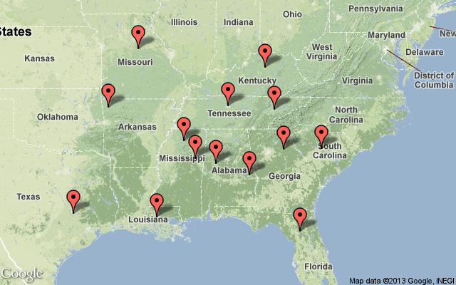
What we need is the minimum road network that connects all these stadiums.

This is a classic graph problem.

Graphs are everywhere

A graph is just a set of objects, called vertices, any two of which are either connected by an edge or not. When you draw one on paper, it looks like one of these:

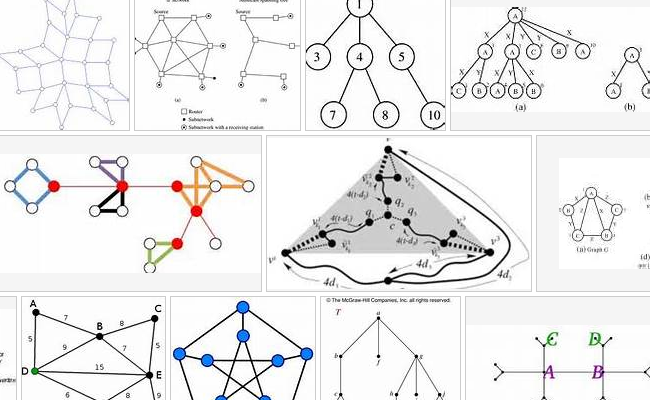
But they’re not just silly math pictures. Interesting real-world relationships can be seen as graphs.

The people of Nashville are the vertices of a graph, where edges connect acquaintances.
A DOM document is a graph, with edges connecting each node to its parent.
All the actors in IMDB are the vertices of a graph, with edges connecting actors who have appeared in a movie together. (Or, all the movies are vertices, connected by common actors. A different graph from the same data.)
All the possible snapshots of a game of chess form an enormous graph, with edges connecting each snapshot with those showing how it might look after the next move.

Food webs, economies, maps, family trees, class hierarchies, the Internet—it’s all graphs. So what? Why do we care? Because there are some powerful practical algorithms that can be applied to all graphs.

Depth-first search is a simple algorithm for finding a path from one vertex to another.
Breadth-first search finds the shortest path. Either algorithm can also be used with minor changes to figure out if a graph contains any cycles.
Dijkstra’s algorithm finds the lowest-cost path from one node to another in a graph where each edge is labeled with a cost.

And if you’re staring down the barrel of total societal collapse and longing for the simple pleasures of the gridiron, you might find Prim’s algorithm useful. It finds a minimum spanning tree: that is, the lowest-cost subgraph of a labeled graph that still connects all the vertices.

The plan

Prim’s algorithm is very simple. It builds the optimal network one edge at a time.

Start with one vertex (any vertex, doesn’t matter) and no edges.
Find the cheapest edge connecting any already-reached vertex to any not-yet-reached vertex.
Add that edge and the new vertex to the network.
If all vertices have been reached, you’re done. Otherwise go back to step 2.

That’s it. Wikipedia gives a simple proof, in case you aren’t convinced that this algorithm always gives a correct answer.

The code

(Full source.)

Start with delicious raw data.

raw_data = [
    ("Florida",  "Gainesville, FL", "Ben Hill Griffin Stadium", 29.6500583, -82.3487493),
    ("Georgia",  "Athens, GA",      "Sanford Stadium",          33.9497366, -83.3733819),
    ("Kentucky", "Lexington, KY",   "Commonwealth Stadium",     38.0220905, -84.5053408),
    ("Missouri", "Columbia, MO",    "Faurot Field",             38.9359174, -92.3334619),
    ...
]

coordinates_by_name = {uni: (lat, long) for uni, _, _, lat, long in raw_data}

Stir in a formula for the distance between two points on the globe.

# Radius of the earth in miles.
earth_radius = 3956.6

def distance(u1, u2):
    return earth_radius * arclen(coordinates_by_name[u1], coordinates_by_name[u2])

# Actual driving distance is 345 miles; as the crow flies, 302.9.
assert 300 < distance("Florida", "Georgia") < 305

And now the main event. Note that the code below works for any distance function you care to provide; it doesn’t have to be based on geographic distances.

def treeify(vertices, distanceFn):
    """ Return a list of triples (distance, v1, v2), the edges of a minimum spanning tree. """

    # This function implements Prim's algorithm:
    # https://en.wikipedia.org/wiki/Prim%27s_algorithm
    # We're going to build a tree. It is initially empty.
    tree_edges = []

    # `unreached` is the set of all vertices our tree hasn't reached yet, which
    # initially is all of them.
    unreached = set(vertices)

    # We'll begin by picking one vertex--it doesn't matter which one--and
    # putting it in our tree. This is the seed from which our tree will grow.
    seed = unreached.pop()

    # We use `edges` to select which edge to add next. Since the algorithm has
    # us repeatedly choosing the cheapest edge, we'll use a heap. Initially it
    # contains all edges leading out from `seed`.
    edges = []
    for v in unreached:
        heapq.heappush(edges, (distanceFn(seed, v), seed, v))

    # When no vertices are left unreached, we'll be done.
    while unreached:
        # Choose the cheapest edge remaining in `edges`.
        new_edge = d, x, y = heapq.heappop(edges)

        # `new_edge` might connect two already-reachable vertices; in that
        # case, skip it and try another. We know that `x` at least is in the
        # tree, since we've only ever added edges leading from inside the tree.
        assert x not in unreached
        if y in unreached:
            # Great, we have the cheapest edge that reaches a new vertex, as
            # required.  Add `y` and `new_edge` to the tree, and add to `edges`
            # all the edges leading from `y` to unreached vertices.
            tree_edges.append(new_edge)
            unreached.remove(y)
            for w in unreached:
                heapq.heappush(edges, (distanceFn(y, w), y, w))

    return tree_edges

42 lines of code, thoroughly commented.

Using this function on the SEC data set is a piece of cake:

import sec, pprint
result = treeify(sec.names, sec.distance)
pprint.pprint(result)
print "Total distance:", sum(row[0] for row in result)

The resulting map:

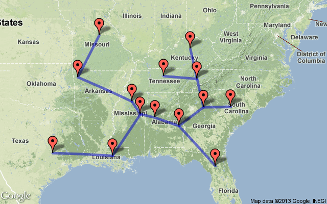
This tree requires the SEC to hold 2,359 miles of road. Source code.

Can we do better?

We made one unnecessary assumption here: namely, that every path had to be a straight line beginning at one stadium and ending at another.

Next week I’ll remove that assumption and see if we can find an even better SEC road network. See you then.

P.S. Kudos to the NCAA on the long-overdue treeification of the college football postseason.